

Time series for each month are stored under $TSDIR/cts/work/$EXPID/post/YYYY_MM. Time series over the whole simulation period and some statistics are stored under $TSDIR/cts/work/$EXPID/eval/data.
Graphics are stored in the directory $TSDIR/cts/work/$EXPID/eval/graphics. For the reference simulation only the area biases are calculated because all other plots show the differences between two simulation. The directory $TSDIR/cts/work/$EXPID/eval/graphics/masks contain the area masks for several European sub regions. These masks are used to cut out the sub regions from the original data.
The following parameters are taken into account for the evaluation:
PMSL
mean sea level pressure
T_2M
two meter temperature
TMIN_2M
two meter minimum temperature
TMAX_2M
two meter maximum temperature
TOT_PREC
total precipitation
The following evaluations are plotted:
R-script:
area-bias.Rs
Calculation:
The annual and seasonal means already calculated with CDO commands during the simulation by the eval.job.tmpl script are used. For temperatures the different orographies of CCLM and observations are taken into account The mean sea level pressure units are transformed from Pa to hPa.
Plot files:
PARAMETER_mm_tm_bias.pdf (PARAMETER is PMSL, T_2M, TMAX_2M, TMIN_2M) PARAMETER ms tm bias.pdf (PARAMETER is TOT_PREC)
Example:
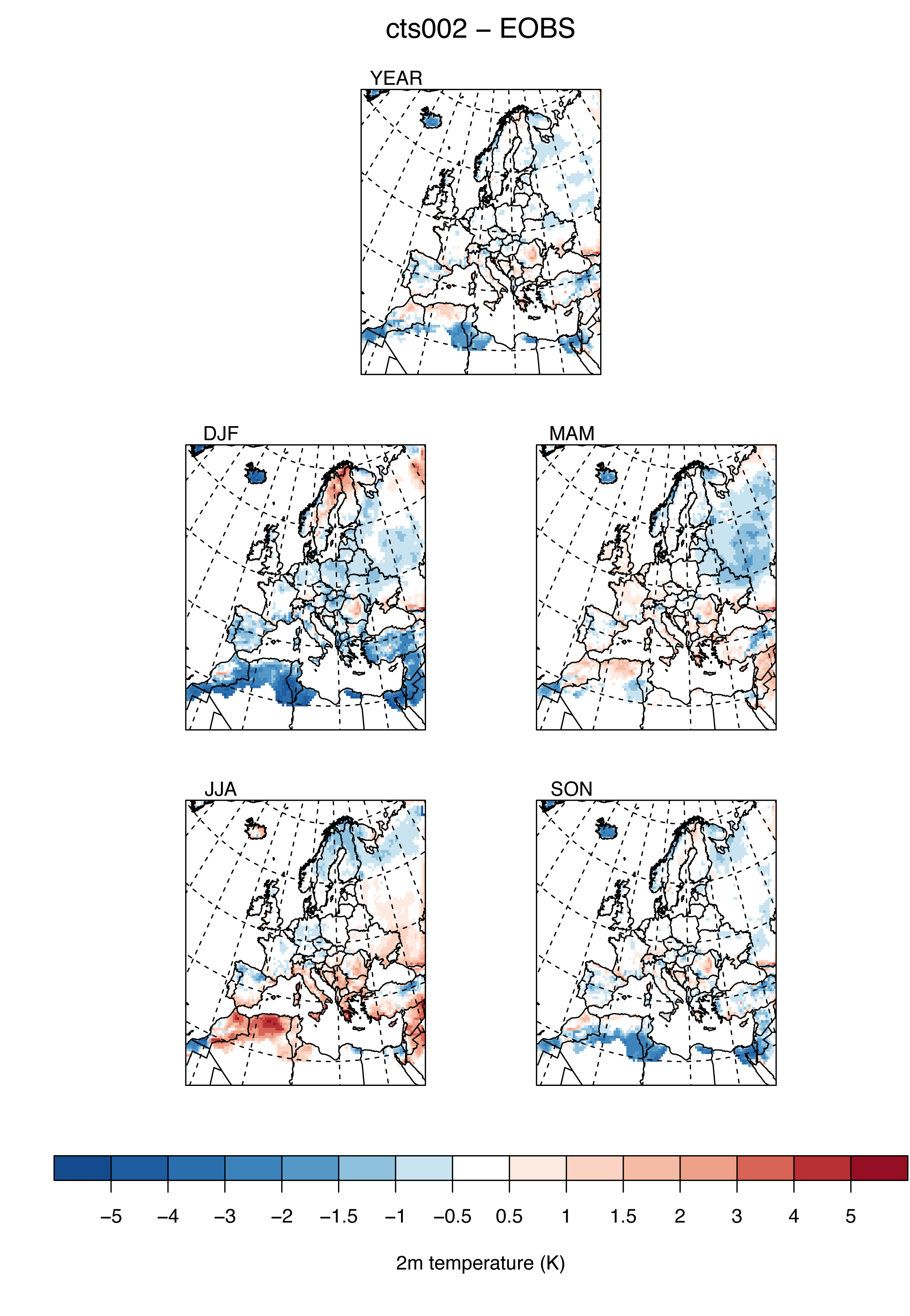
R-script:
annual-cycle-bias.Rs
Calculation:
Annual monthly means are calculated with cdo ymonmean on the basis of the monthly mean and sums calculated during the simulation by the eval.job.tmpl script. For temperatures the different orographies of CCLM and observations are taken into account The mean sea level pressure units are transformed from Pa to hPa.
Plot files:
PARAMETER_annual_cycle_bias.pdf (PARAMETER is PMSL, T_2M, TMAX_2M, TMIN_2M, TOT_PREC)
Example:
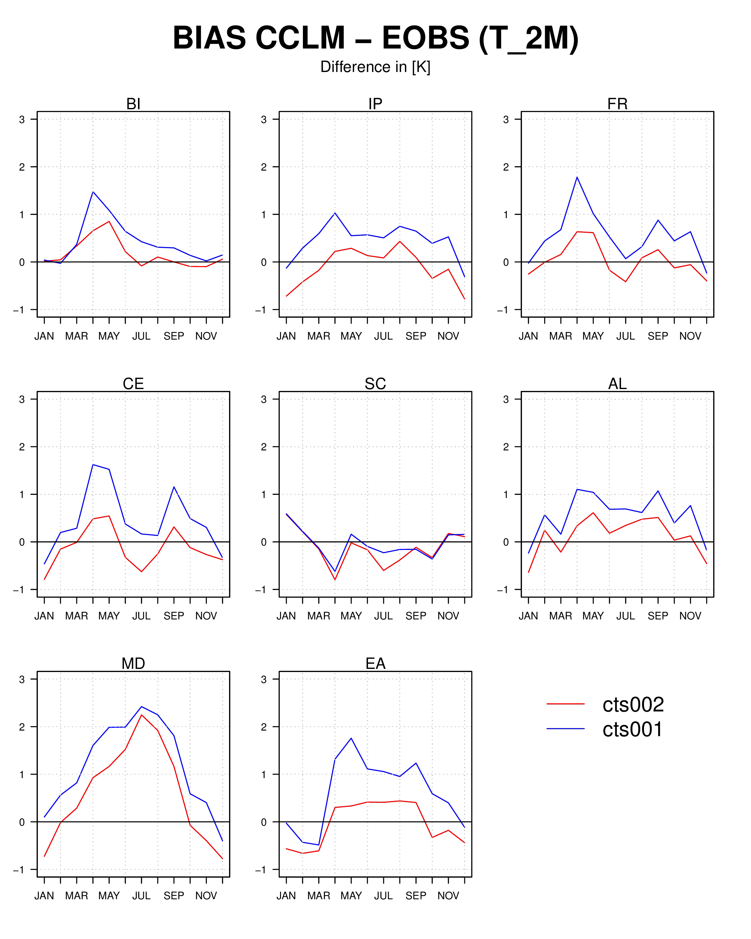
R-script:
taylor-diagram-spatial.Rs
Calculation:
Mean over all years and mean over all the years for each season are calculated with
Plot files:
PARAMETER_taylor_spatial.pdf (PARAMETER is PMSL, T_2M, TMAX_2M, TMIN_2M, TOT_PREC)
Example:
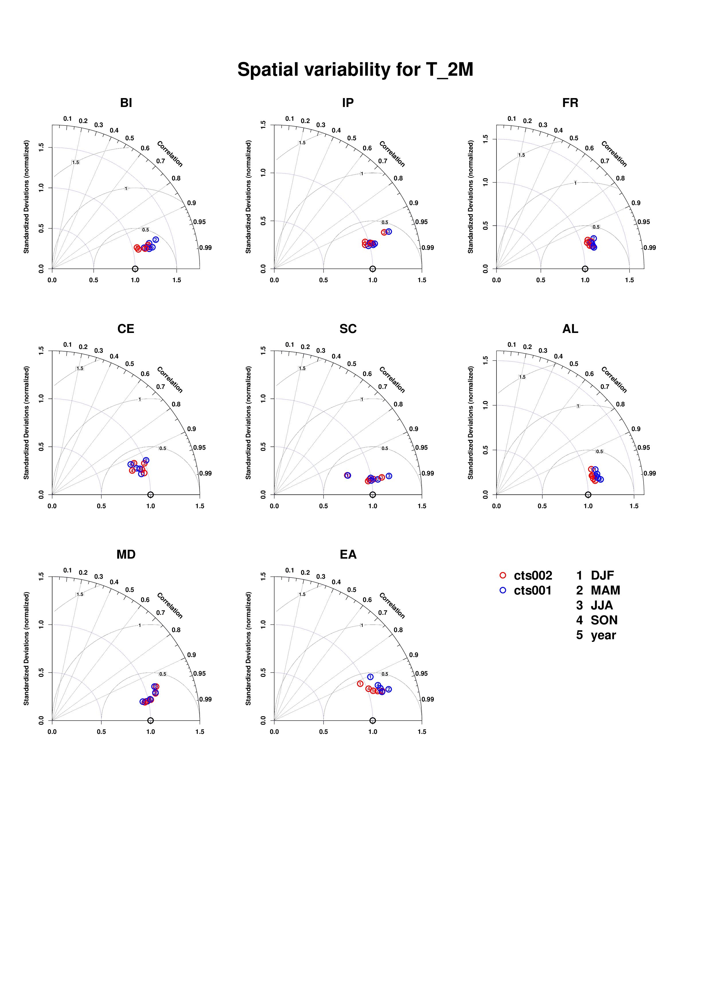
taylor-diagram-spatial.Rs
Calculation:
Mean over all years and mean over all the years for each season are calculated with
cdo timmean -selmon. The taylor diagram is plotted with the taylor.diagram script of the plotrix R package. For a better quality ghostscript is used to convert the plot.Plot files:
PARAMETER_taylor_spatial.pdf (PARAMETER is PMSL, T_2M, TMAX_2M, TMIN_2M, TOT_PREC)
Example:
R-script:
taylor-diagram-temporal.Rs
Calculation:
Mean over European sub regions are calculated with
Plot files:
PARAMETER_taylor_temporal.pdf (PARAMETER is PMSL, T_2M, TMAX_2M, TMIN_2M, TOT_PREC)
Example:
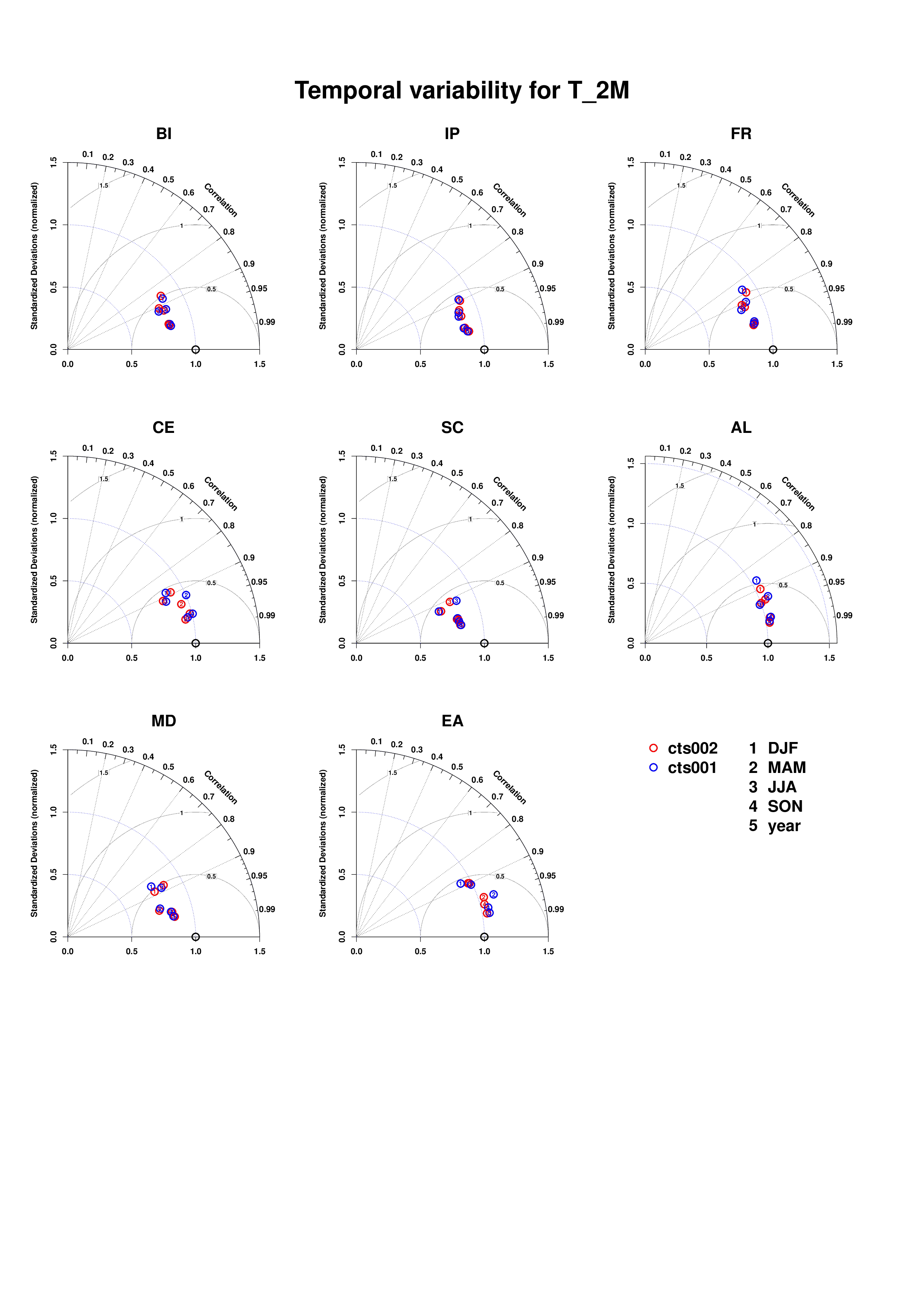
taylor-diagram-temporal.Rs
Calculation:
Mean over European sub regions are calculated with
cdo fldmean -selmon. The taylor diagram is plotted with the taylor.diagram script of the plotrix R-package. For a better quality ghostscript is used to convert the plot.Plot files:
PARAMETER_taylor_temporal.pdf (PARAMETER is PMSL, T_2M, TMAX_2M, TMIN_2M, TOT_PREC)
Example:
R-script:
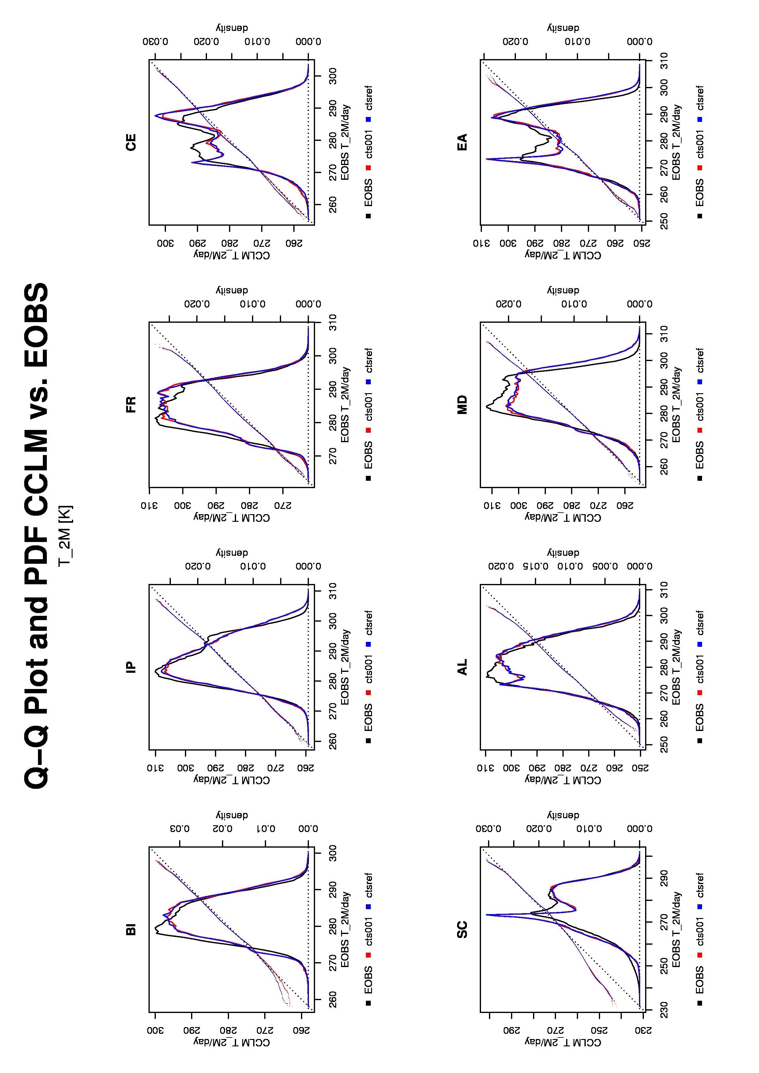
qq_pdf.Rs
Calculation:
For the qq-plot the results of the simulations and the observations are sorted by their values. All grid points in space and time are taken into account. The sorted data are then plotted as simulations versus observations.
For the pdf-plot histograms are calculated with the hist script of the graphics R-package. The script gives the number of counts in each histogram interval. The number of breaks defining there intervals are calculated by the following R commands:
where the variable param.hist.break[iparam] hold the constant width of the intervals. These widths are defined for the different quantities as follows: PMSL(100Pa), T 2M(0.5K), TMIN 2M(0.5K), TMAX 2M(0.5K), TOT PREC(1.mm).
The number of counts in each interval is divided by the total number of counts. These normalized data are then plotted.
Since there is huge number of point to be plotted which causes a long loading time of the output in PDF format, an additional output file in JPEG format is created by the convert command from the imagemagick program package.
Plot files:
PARAMETER_qq_pdf.pdf (PARAMETER is PMSL, T_2M, TMAX_2M, TMIN_2M, TOT_PREC)
Example:
qq_pdf.Rs
Calculation:
For the qq-plot the results of the simulations and the observations are sorted by their values. All grid points in space and time are taken into account. The sorted data are then plotted as simulations versus observations.
For the pdf-plot histograms are calculated with the hist script of the graphics R-package. The script gives the number of counts in each histogram interval. The number of breaks defining there intervals are calculated by the following R commands:
data.min<-floor(min(data.obs, data.exp, data.ref)/
      param.hist.break[iparam])*param.hist.break[iparam]
data.max<-ceiling(max(data.obs, data.exp, data.ref)/
      param.hist.break[iparam])*param.hist.break[iparam]
tbreaks<-c(seq(data.min,data.max,by=param.hist.break[iparam]))
where the variable param.hist.break[iparam] hold the constant width of the intervals. These widths are defined for the different quantities as follows: PMSL(100Pa), T 2M(0.5K), TMIN 2M(0.5K), TMAX 2M(0.5K), TOT PREC(1.mm).
The number of counts in each interval is divided by the total number of counts. These normalized data are then plotted.
Since there is huge number of point to be plotted which causes a long loading time of the output in PDF format, an additional output file in JPEG format is created by the convert command from the imagemagick program package.
Plot files:
PARAMETER_qq_pdf.pdf (PARAMETER is PMSL, T_2M, TMAX_2M, TMIN_2M, TOT_PREC)
Example:
R-script:
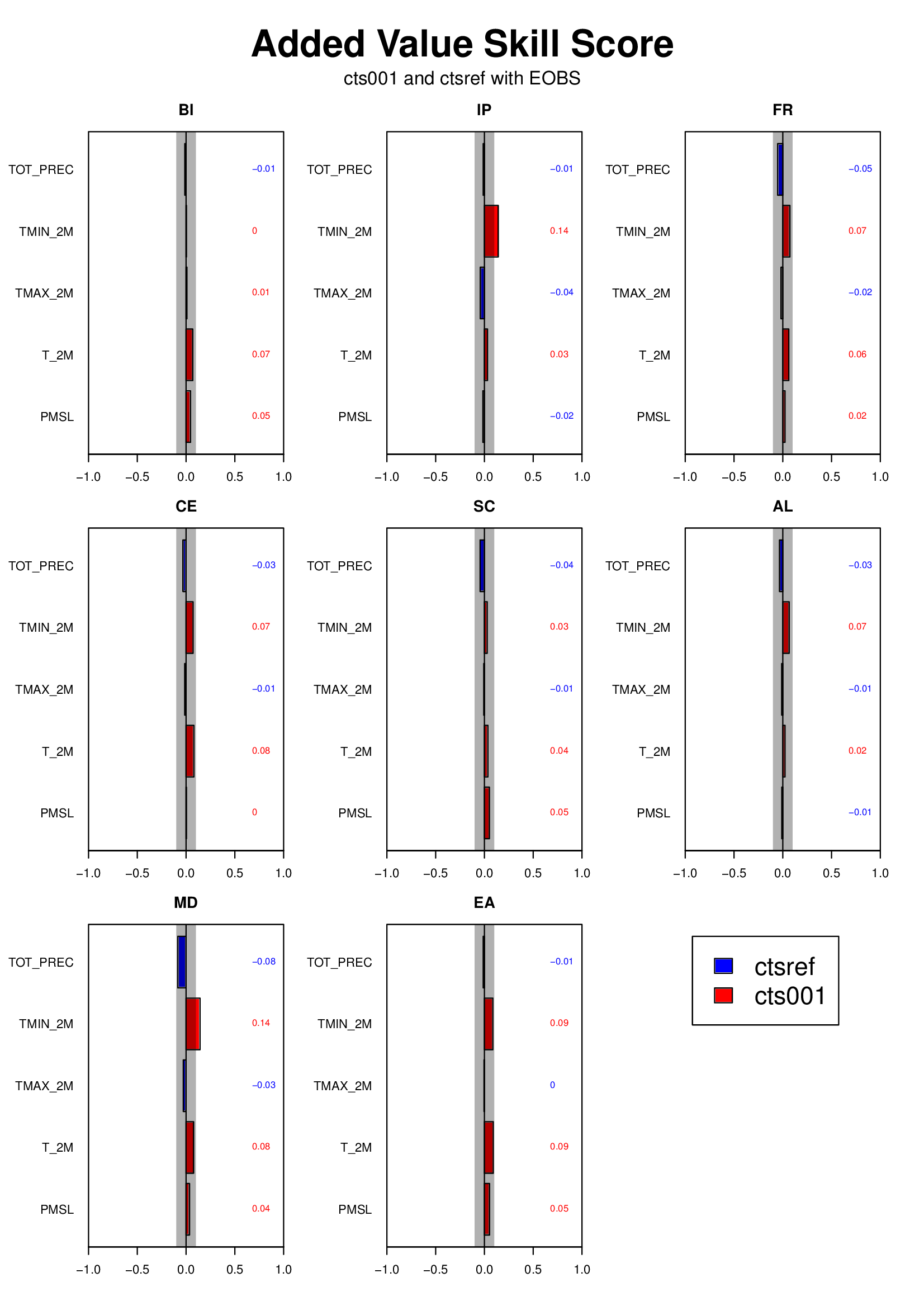
avss.Rs
Calculation:
The added value skill score is calculated by
$$AVSS=\left\{\begin{matrix} 1. -\frac{RMS_{obs-test}}{RMS_{obs-ref}} & \frac{RMS_{obs-test}}{RMS_{obs-ref}} \le 0 \\ 1.-\frac{RMS_{obs-ref}}{RMS_{obs-test}} & \frac{RMS_{obs-test}}{RMS_{obs-ref}} > 0 \end{matrix}\right.$$
Plot files:
avss.pdf
Example:
R-script:
pss.Rs
Calculation:
The difference between two probability density functions is calculated by
where n ist the total number of data point (i.e. the sum over the pdf) and m is the total number
of histogram bins.
Plot files:
pss.pdf
Example:
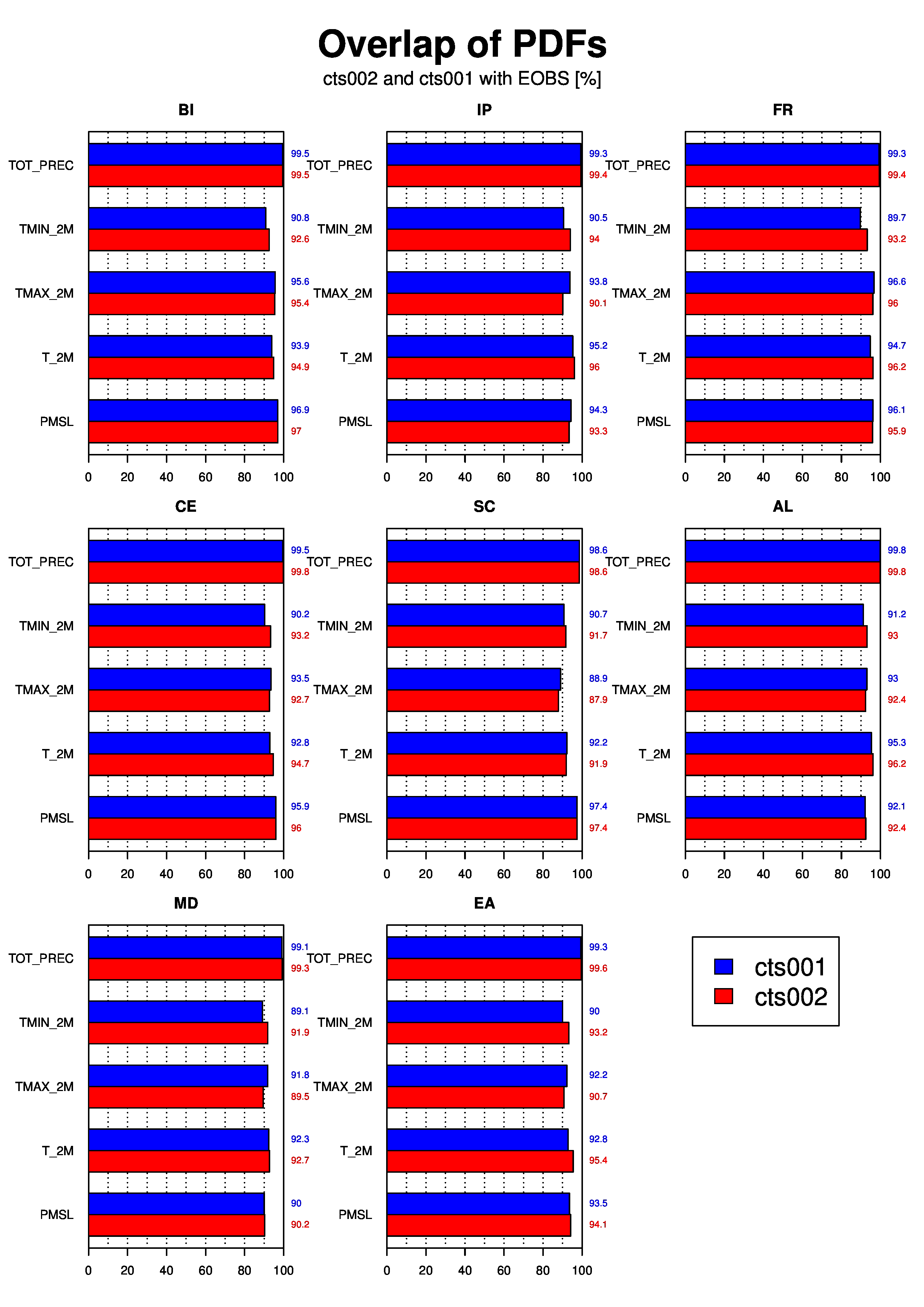
pss.Rs
Calculation:
The difference between two probability density functions is calculated by
- creating a the pdf as a histogram (see section “QQ and PDF” above)
- calculate the overlap from the histogram as follows in percent:
where n ist the total number of data point (i.e. the sum over the pdf) and m is the total number
of histogram bins.
Plot files:
pss.pdf
Example:
Page last updated: 17.12.18